Visualizing TCR repertoires with UMAP
Dimensionality reduction with Parametric UMAP
The CDR3 hashing described above generates 64-dimensional fingerprints of CDR3 sequences. Reducing this dimensionality allows us to map and visualize the full scope of CDR3 diversity.
Parametric UMAP is a parametric form of the uniform manifold approximation and projection (UMAP) algorithm. Both methods have the same objective: creating a low-dimensional projection of a high-dimensional dataset, while preserving the underlying topological structure. UMAP does this in two steps: first compute a graph representing the data, then learn an embedding from that graph. Parametric UMAP additionally employs a neural network to directly learn how the data maps to the embedding. In terms of speed, training this neural network is slower than just performing a UMAP. However; once trained, new (unseen) datapoints can be directly transformed by feeding them through the neural network, which is orders of magnitude faster than reapplying UMAP.
Usage
Training a Parametric UMAP transformer
An unbiased training set of 250000 CDR3 sequences was generated using the generative model of VDJ recombination implemented by OLGA.
./generate_sequences.py --humanTRB -n 250000 > olga_TRB.tsv
These sequences were read in:
from raptcr.readers import read_AIRR
data_train = read_AIRR('~/UA/databases/mixcr_airr_example.tsv')
A CDR3 hasher was fitted as earlier described.
from raptcr.hashing import Cdr3Hasher
cdr3_hasher = Cdr3Hasher(pos_p=0.5, clip=1)
In this example, we will make use of early stopping to avoid overfitting and speed up training. For this, we need to additionally provide keras_fit_kwargs, containing following arguments. For more info read the documentation here.
import tensorflow as tf
keras_fit_kwargs = dict(
        callbacks=tf.keras.callbacks.EarlyStopping(
        monitor='loss',
        min_delta=0.002,
        patience=3,
        verbose=1,
    )
)
Finally, we can train the Parametric UMAP transformer. This will take a while!
from raptcr.visualize import ParametricUmapTransformer
pumap = ParametricUmapTransformer(hasher=hasher, keras_fit_kwargs=keras_fit_kwargs)
pumap.fit(data_train)
Fri Nov 25 14:40:59 2022 Construct fuzzy simplicial set
Fri Nov 25 14:40:59 2022 Finding Nearest Neighbors
Fri Nov 25 14:40:59 2022 Building RP forest with 30 trees
Fri Nov 25 14:41:03 2022 NN descent for 18 iterations
	 1  /  18
	 2  /  18
	 3  /  18
	 4  /  18
	 5  /  18
	 6  /  18
	Stopping threshold met -- exiting after 6 iterations
Fri Nov 25 14:41:23 2022 Finished Nearest Neighbor Search
Fri Nov 25 14:41:26 2022 Construct embedding
Epoch 1/100
33718/33718 [==============================] - 637s 19ms/step - loss: 0.1519
Epoch 2/100
33718/33718 [==============================] - 625s 19ms/step - loss: 0.1409
Epoch 3/100
33718/33718 [==============================] - 595s 18ms/step - loss: 0.1394
Epoch 4/100
33718/33718 [==============================] - 564s 17ms/step - loss: 0.1386
Epoch 5/100
33718/33718 [==============================] - 575s 17ms/step - loss: 0.1379
Epoch 6/100
33718/33718 [==============================] - 516s 15ms/step - loss: 0.1377
Epoch 7/100
33718/33718 [==============================] - 524s 16ms/step - loss: 0.1374
Epoch 00007: early stopping
7813/7813 [==============================] - 5s 592us/step
Fri Nov 25 16:01:28 2022 Finished embedding
… and save the final model. Provide a path to a folder where the model will be saved.
pumap.save('./trained_model')
The pretrained UMAP transformer can be downloaded from the examples directory in the RapTCR github. Nevermind, its 500mb and github thinks thats too big.
Using the ParametricUmapTransformer
We provide an alternative constructor to read a saved transformer from file.
pumap = ParametricUmapTransformer.from_file("./trained_model")
Lets apply it on an unseen dataset:
data = read_AIRR('~/UA/databases/mixcr_airr_example.tsv')
result_df = pumap.transform(data)
This adds x and y coordinates to our data, returning a dataframe.
| sequence_id | v_call | j_call | junction_aa | x | y | duplicate_count |
|---|---|---|---|---|---|---|
| clone.1 | TRBV7-2*00 | TRBJ2-7*00 | CASSSPGREYDYEQYF | 11.7696 | 10.0269 | 4051 |
| clone.7 | TRBV19*00 | TRBJ2-7*00 | CASSITPGQGTDEQYF | 10.787 | 11.5674 | 1615 |
| clone.8 | TRBV2*00 | TRBJ1-4*00 | CASIYQGSEKLFF | 12.9176 | -5.69044 | 1480 |
| clone.10 | TRBV24-1*00 | TRBJ2-2*00 | CATYDGNTGELFF | 13.2503 | -4.71584 | 1151 |
| clone.12 | TRBV29-1*00 | TRBJ2-1*00 | CSVDWPKNEQFF | 7.26848 | 6.42463 | 991 |
This transformation is really fast:
%%timeit
pumap.transform(data)
119 ms ± 7.21 ms per loop (mean ± std. dev. of 7 runs, 10 loops each)
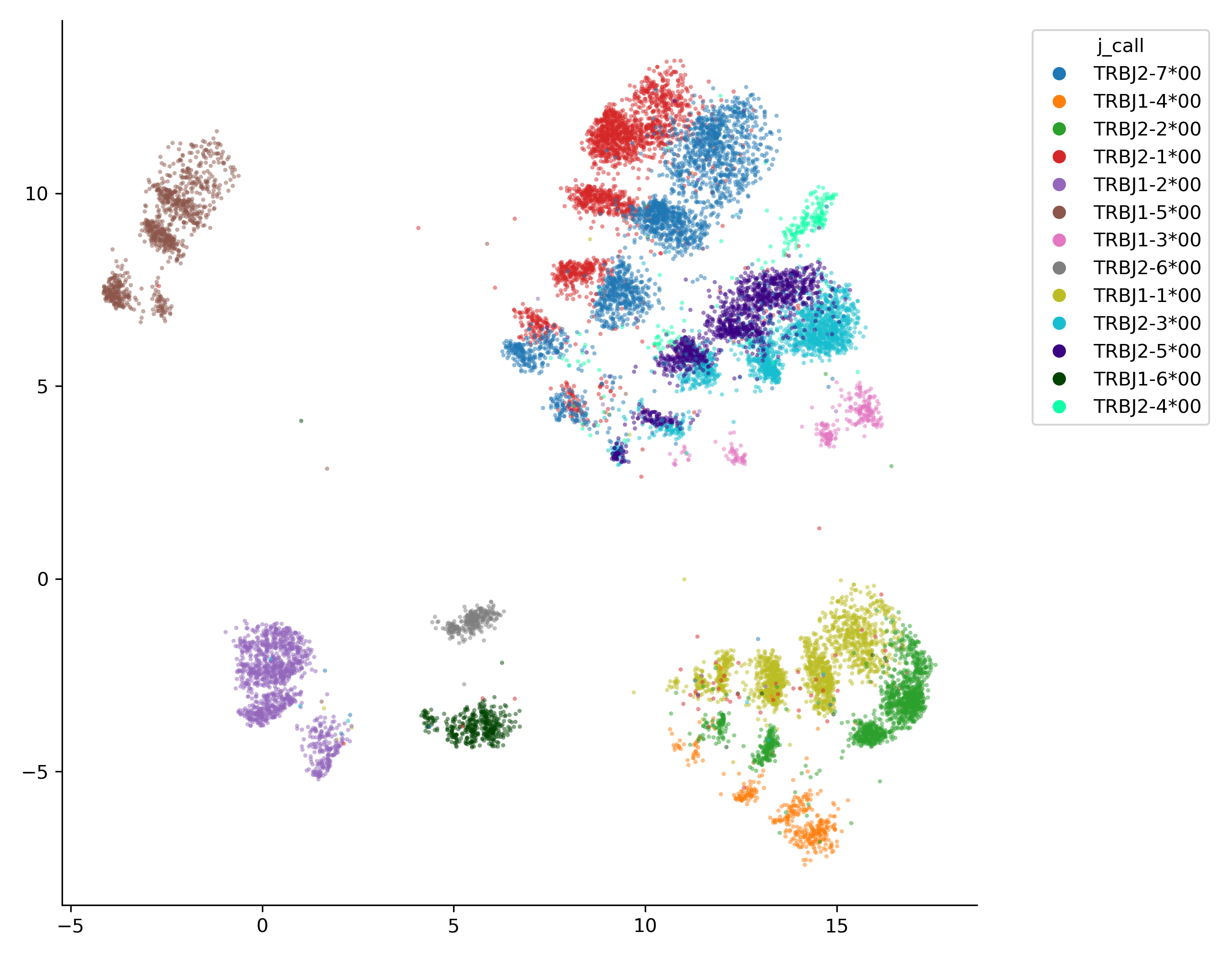
You can now use these UMAP coordinates to visualize the dataset with your method of preference. An easy matplotlib-based class is provided in the raptcr.visualize module:
from raptcr.visualize import ParametricUmapPlotter

# create a figure and axes object
fig, ax = plt.subplots(figsize=(7,7))

ParametricUmapPlotter(df).plot(
    ax=ax, #the axis to plot on
    color_feature = "j_call", #the df column used to color the points, can be numeric or categorical
    plot_legend=True,
)

plt.tight_layout()
plt.savefig("examples/example_UMAP.png", dpi=300)
